Building a Neural Network in Go

Creating a multi-layer perceptron from scratch with just the Go standard library.

December 12, 2021

This post covers the creation of a multi-layer neural network written in Go. We will walk through the basics of what neural networks are and how they work, specifically looking at some of the earliest types of feed-forward neural networks. We will then walk through the implementation of a Multi-Layer Perceptron (MLP). Our goal in this process is to create a network that performs well at recognizing handwritten digits on the MNIST dataset.

Neural networks are at the heart of most recent advancements in machine learning systems, but the fantastic ecosystem of libraries and tools available to implement and experiment with them can obscure the inner details of how they function. This post goes into the full details of how basic feed-forward neural networks function, aiming to give a concrete understanding of the details as a foundation for more deeply engaging with the current state of the field.

While there are a number of resources available that cover either the implementation of basic single layer networks or the concepts and math behind neural networks generally, there seems to be scant resources available online which cover both concept and implementation of multi-layer networks, particularly in a way that goes into the details of backpropagation and structuring it to be flexible enough for a variety of use cases. Our goal here is to use the process of implementing the network from top to bottom to get a “full stack” understanding of these networks, limiting ourselves to using just the Go standard library so that the mathematical pieces are all laid out as well.

While we will be implementing this network from scratch, I’ll be linking out to other fantastic resources that can provide further detail on the various implementation aspects of the network, including a deeper walk through of the concepts and intuition behind neural networks and more detail on deriving back-propagation.

This is a fairly long post, so do feel free to expand the table of contents above and skip around!

The network that is created over the course of this post can be found here: github.com/kujenga/goml. Snippets throughout the post will link out to relevant sections as we walk through the implementation there.

What is a neural network?

Neural networks are a type of machine learning system that is modeled after a basic understanding of the human brain. They are made up of sets of neurons, each of which performs basic compute functions to its inputs and passes on its “activations” to subsequent neurons in the network. The network as a whole thus is a set of inputs and produces a set of output predictions as the “activations” of the final layer, the result of the values passing through the network neurons.

A single-layer Perceptron is the simplest useful network, the idea for which was first introduced in 1958! It can solve basic linearly separable problems, meaning that you could draw straight line(s) to bisect the different categories in the output.

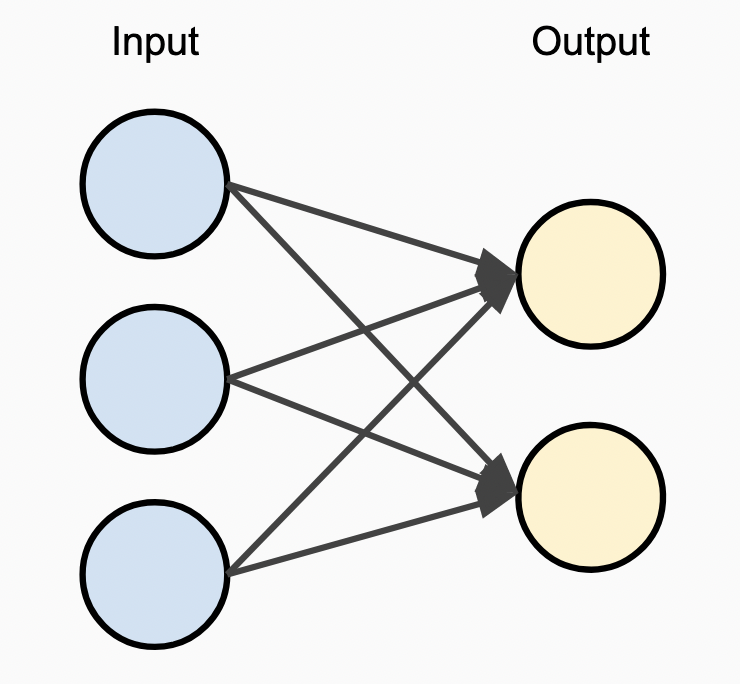
The diagram to the right illustrates the basic structure of a single-layer perceptron. Inputs come in on the left-hand side of the network, are passed to the next layer via the edges represented with directional lines, and are passed into the output nodes that represent the predictions of the network. As we’re looking at this diagram, one thing to note is that the real magic of the network is mostly all in the edges themselves. The nodes within the input layer basically just relay values into the network, and the method by which we propagate those values to the following layers is where the actual computation happens.

While naming conventions for neural networks can be used in different ways, perceptrons are generally thought of as a sub-class of feed-forward neural networks, where the neurons are organized into a series of discrete layers, with activations from one layer passed as inputs to the next.

Understanding neurons

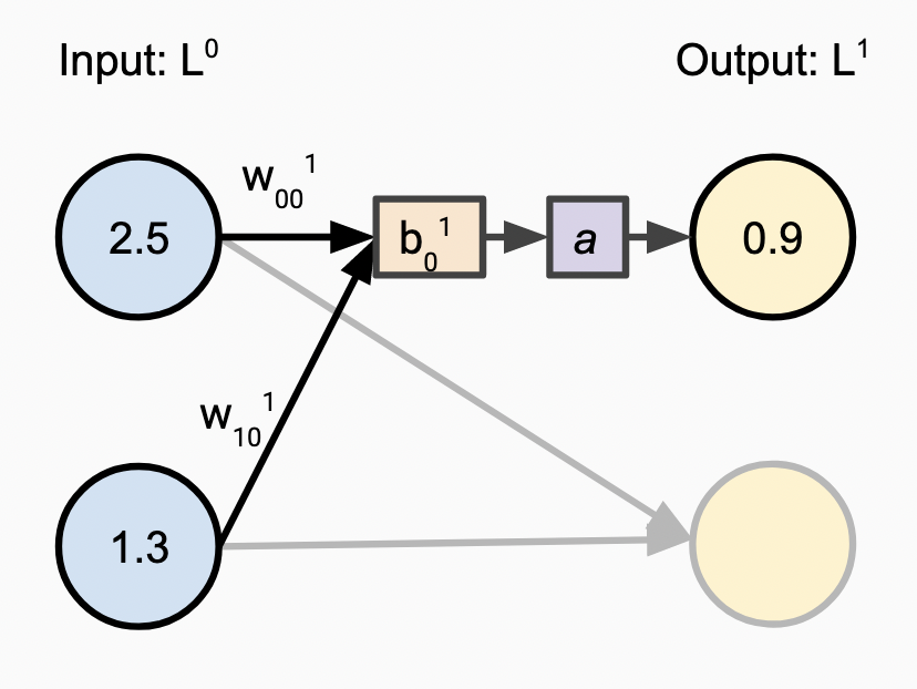
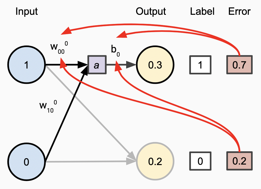
Each of the nodes in the above graph is often referred to as a “neuron”, as they are intended to roughly mimic the structures within a simplified model of the brain. Let’s dive a bit deeper into how these artificial neurons, and more importantly the edges between them, function. The image below illustrates each of the following steps.

One note on that diagram is that by convention, edges and their corresponding weights belong to the nodes that the directional arrows are pointing to. In this diagram we are looking at layer $L^{1}$, where layer $L^{0}$ is the input layer which simply passes values forward without computation.

First we define weight parameters $w_{j,k}^{(l)}$ for each layer of the network $l$, where $j$ is the index of the node in the previous layer $l - 1$, and $k$ is the index of the node in the current layer $l$.
Next, for each node in the current layer $L^{1}$ (the input layer is always skipped), we take the sum of the values from the prior layer, multiplied by the weights on each corresponding edge.
We then add a bias $b_{k}^{(l)}$ to the weighted value, shifting it one way or the other.
Now we apply an “activation function” $a$ to the prior result, which adds non-linearity and enables us to build a network with more than a single layer¹.
If this is the last layer in the network, the resulting values are the predictions made by the network! Otherwise, they are passed on to subsequent layers and this process is repeated.

Here we see these steps laid out with specific example values to illustrate the process:

Activation Functions

Logistic Curve — By Qef, Public Domain, https://commons.wikimedia.org/w/index.php?curid=4310325

A key element of the above diagram is the activation function that modifies the combination of the incoming values, weights, and biases. Activation functions are non-linear functions that transform these values in a way that gives the network more expressive power. Without the addition of a non-linear component in the network we just have a series of linear transformations, which limits the types of problems we can solve.

In our network implementation we will be using a logistic activation function, also known as sigmoid, which is displayed in the diagram to the right. The output is represented on the y-axis and the input on the x-axis. The smoothing of more extreme input values is critical to the learning ability of the network.

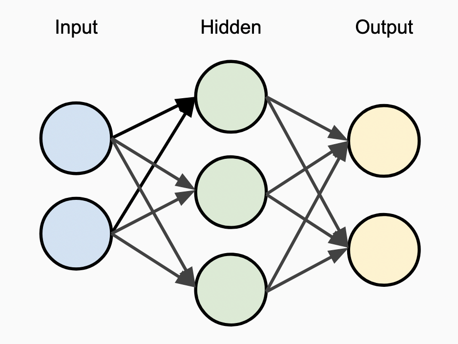
Adding layers to the network

To make this network more capable, we can extend the model of a single-layer perceptron by adding more layers, creating a multi-layer perceptron. The number and size of layers in this network are referred to as as the “network architecture”, and such configurations values are often referred to as “hyperparameters” defining the architecture. As in the single-layer example, the first layer in the network is termed out “input” layer, and the last layer in the network is termed our “output” layer. The new interior layers are commonly referred to as “hidden” layers, as they are internal to the network.

More layers add capabilities to the network and facilitate much more complex use cases. The ability to add in hidden layers will be instrumental in tackling the MNIST dataset.

In the rest of this post, we will build out an implementation of Multi-Layer Perceptrons in this style that is flexible with respect to the network architecture, allowing for an arbitrary number of layers at arbitrary sizes.

Let’s build

As we mentioned in the intro, at their most basic level neural networks take in a set of inputs and produce a set of outputs. In the process of constructing a network, we can center our development around a basic set of unit tests that validate this behavior. We’ll use two basic classes of tests, one to verify our ability to learn the outputs of common boolean functions, and then later on we’ll add test cases to train and predict handwriting recognition on the MNIST dataset.

Boolean test cases

Before we get into the MNIST problem, we want to start with super simple, to check that our network can do anything at all. The setup I am using for that level of verification in this post is the ability for an individual network to learn basic boolean functions like AND and OR.

Here is an example of the basic test cases we will build on for the boolean inputs and the corresponding output labels that different instantiations of the network can learn.

We define these using a lin.Frame type that represents a 2D Matrix of data. Our [lin] package will be used to capture various types to help with the linear algebra involved in network creation. The first declaration is the set of all possible inputs for two boolean values. The subsequent declarations outline different types of boolean functions. Each of these functions is something that a different instantiation of a network will be able to iteratively learn.

MNIST test cases

In contrast to these examples of replicating basic boolean logic, the MNIST dataset is a real machine learning problem where you must create a way to predict the digit between 0-9 corresponding to an image of a hand-written number, a very simple form of optical character recognition. This dataset is a great example of where a basic neural network performs well relative to other approaches, and is one of the classic datasets for training models on.

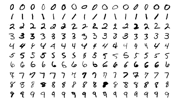
One caveat here is that the MNIST dataset distributed in a unique binary format, which we will need to de-serialize in order to make use of it in a test case. We will walk through that later in the post. Each of the digits seen in the image below is an example from the dataset, represented as a 28x28 pixel image, with values in integer form from 0-255. To pass the data into the model we’ll need to represent this as an array, and normalize the values into floating point numbers better suited for transformation.

MNIST Examples — Josef Steppan, CC BY-SA 4.0 <https://creativecommons.org/licenses/by-sa/4.0>, via Wikimedia Commons

Code structure

As we think about how to structure the code for our network, there are a few key pieces of functionality we need to provide:

Initialize the network, allocating the needed data structures and initial values.
Train the network, iteratively improving the network output based on inputs.
Make predictions using the trained network, taking a set of inputs and providing a computed output.

In addition to these basic functionalities, we also want to build it in a flexible manner that can facilitate any number of layers. By doing so, we can create networks of different architectures to facilitate different use cases. This may also facilitate iterations to support more complex types of neural networks, a possible topic for future posts.

For this implementation we will favor clarity and readability over efficiency optimizations, aligned with the goal of this project as a way to learn the details of how networks operate.

Starting off, the primary struct controlling our network is the MLP struct, representing our Multi-Layer Perceptron, and is fairly simple. It holds an array of layers that form the structure of the network and hold state for training and prediction. The LearningRate variable is a network-level hyperparameter controlling the training process which we’ll look at more closely later, and the Introspect function allows us to look at incremental training progress.

Diving deeper into the implementation, the Layer struct represents a single layer within our feed-forward network. Here things start to get more complex, as there is quite a bit of state that needs to be managed to facilitate the entirety of the training process.

The key elements to capture within this data structure are:

Parameters that define the layer behavior, including the width of the network and the activation function.
Internal references to the network itself, as well as the next and previous layers in the network. We need references in both directions to facilitate forward and backward propagation.
Internal state values of the layer, holding the weights and biases. We’ll look at how these are used more closely in the next section.
Records of the internal activation values that the layer had last seen. These need to be captured for use in the backpropagation training process.

With these two structures defined, we can look at how the training process works. The entry point is the Train function, which iterates for a given number of epochs. Each epoch is a pass over the entire dataset. Training happens iteratively, with each step containing two passes.

For each input, we first propagate the weights and subsequent layer outputs forward through the network to get the current predictions of the network for the given input. Once that is complete, we propagate the error values we compute based on the corresponding labels backwards though the network, and update the weight parameters within the network in a way that would have reduced the error we saw for that given input.

Bear with me here, as we will dive into the details of what those crucial ForwardProp and BackProp functions are doing in detail momentarily.

Once the network is trained with the above method, we can use it for making predictions! There is some neat symmetry in the implementation here, as the Predict function is identical to the first part of the inner loop of the Train function where we are propagate our inputs forwards through the network.

One note on this approach is that the float32 type was chosen as full float64 precision isn’t needed here. Many state of the art ML platforms are using even lower precision for increased memory efficiency, or even delving into “mixed precision” schemes² that combine multiple precision levels as needed. When Go adds support for generics³ this value could be something made configurable.

Next we’ll look at how the network internals are initialized, and then dive in the details of forward and backward propagation.

Initialization: data structures for learning

Neural networks require a lot of internal state that holds network parameters that encode the predictive power of the network, as well as temporary values used in the training process. Here we’ll look at what those values are and how we set them up.

Initialization of the MLP as a whole is done with a basic iteration over the layers, initializing each one as shown here. As we’ll see later on, the pointers to the previous and next layers are critical in the training process, so those are passed in at this point in time to connect the layers together.

The initialize function on each layer performs the bulk of the setup work for the network. First, we initialize the basic pointers to network state, keeping track of the MLP itself as well as the passed in next and previous layers, as well as configuring a default activation function and it’s corresponding derivative if they were not already specified.

With those basic values in place, we move on to initializing the data structures for the network’s internal parameters. Here we initialize the weights and biases to random values. To understand why random initial values make sense, I find it helpful to imagine setting all the weights to the same value, say 1.0. In order to train any network, you need to figure out which weights are contributing the most to the resulting error, but if all the weights are the same, you end up in a situations where multiple weights might be able to be tweaked for similar effect. In such cases you can conceptual imagine it being unclear which weights to move in which directions, and this can slow down the overall training process. Another aspect of the initialization is the scaling the weights by the “connectedness” of the node.

To understand why this is helpful, think back to the shape of the sigmoid activation function, shown here again, and what happens as the input “x” values get larger. The “y” values get asymptotically closer and closer to 1.0, and the differences between them get smaller, meaning that changes to the weights have less of an ability to effect the network output, which can make it harder to train and converge. By keeping the weights proportionally smaller, we leverage more of the curved portion of the sigmoid function and give the calculations more discriminative power. It is worth noting that this limitation is somewhat specific to asymptotic activations functions like sigmoid, but it shouldn’t hurt with others that are not.

Lastly, we initialize data structures to keep track of the last seen error (lastE) and loss (lastL) values for the layer, which are a critical component of backwards propagation as we will see later on.

Forward Propagation: Making predictions

We will now be diving into the implementation of the forward propagation step, where we transform a set of inputs passed into a layer of the network into a set of “activation” outputs.

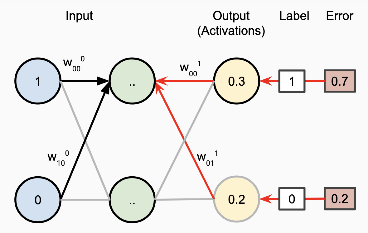
As an aside, one thing I have found confusing in some portrayals of neural networks is that so much of the focus is on the “neurons” themselves, represented as nodes in the network graph. The real magic is all in the edges! The weights attached to the edges, the activation function that they pass through, and the bias values shifting the output, are what give these networks their power. The nodes themselves are really just representations of state, which is what this diagram attempts to show:

In order to turn this structure into code, we iterate through each input value we are receiving from the last layer and calculate the new activations. This is skipped for the input layer, since it is just receiving the raw values into the network and there are no corresponding weights. The combination of the weights and input values into a single value is most clearly expressed as a dot product, and the Z value is used to record the linear combination of the weights with the bias added in before the activation function. Both this Z value and the activation value itself are stored, not for use in the forward propagation, but for use later in the backpropagation training process.

Backpropagation: Training the network

Being able to compute a set of outputs given a set of inputs is a big step forward, but in order to give meaning to these outputs, we need to train the network to match the predictive behavior that we expect. Nearly all machine learning models are trained through a series of iterative steps, where each step tweaks the parameters of the model in a way that decreases the “loss” of the network. We’ll be doing that same process here in our network.

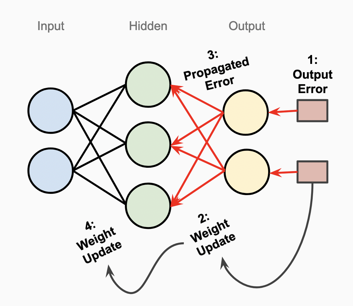
In each iterative step, our goal is to update the weight and bias parameters in the network to minimize the error. Looking now at the diagram below and moving backwards through this three layer network, our conceptual steps are:

Compute the output error by comparing the activation values of the output layer with the truth labels from the dataset.
Update the weights and biases in a way that will decrease the computed error. We do this using derivatives which we will walk through next, which tell us how to move the weights and biases for this to happen.
Continue to propagate different, computed error values backwards through the network, weighting it through the edges that contributed to the output error.
Iteratively update the next set of weights to minimize errors caused by that earlier layer, and repeat as needed for subsequent layers.

If you’d like to go into more depth with understanding the intuition behind backpropagation, watch this video. I found it very helpful in understanding the process: Backpropagation explained | Part 1 - The intuition

Introducing Loss Functions

In the above diagram, we talk about propagating the “error” back through the network. However this presents a slight hiccup, as the simplest way to calculate error values, computing the difference between the expected labeled output and the output we received from the network, can be either a positive or negative value. These values can cancel each other out in undesirable ways when combined. In order to determine how well the network is performing, we need to be able to look at the aggregate of all the errors we observe in the output. We do this using a Loss Function, which transforms the raw error from the network into something more mathematically useful to us.

For our network, we will be using the Mean Squared Error (MSE) loss function, which is just what it sounds like, taking the average of the squared values from each output. By squaring the error values we make them all positive, and the summed errors in the average always correctly indicate that the network is doing better or worse and there is no cancellation. The formula for MSE is as follows:

$$\frac{1}{N} \sum_{i=1}^N (labels_{i} - outputs_{i})^2$$

There are all sorts of different loss function with varying properties which can be used as well. More can be read about different loss functions in other resources around the web⁴.

Understanding Gradient Descent

Now that we have the basic concepts of propagating error values back through the network to update parameters and using loss functions to calculate how well (or poorly) the network is doing, we can apply this process repeatedly to iteratively improve our network’s performance. This iterative process is known as Gradient Descent.

Conceptually, the gradient we are referring to can be thought of as a hilly landscape representing the loss of the network, which we represent here from the top in two dimensions. The vertical axis represents the loss, where lower is better, and the horizontal access represents the space of possible parameters that we can move around within as we look for the point to minimize this loss. In reality, the number of dimensions in this graph is the same as the number of parameters we are trying to tweak, but this conceptual understanding remains valid as the model scales.

In the training process, the goal is to find the point in this landscape that minimizes the loss for the inputs that we care about.

There are a few different approaches to Gradient Descent, but the one we will be starting off with here is the simplest, called Stochastic Gradient Descent (SGD). With SGD, you look at one input at a time from your dataset, and update the network based on the loss from that input/label pair. Other types of gradient descent such as batch and mini-batch look at multiple inputs and label pairs at a time, which can have various advantages⁵, but introduce complexity as well, so we skip those for the scope of this post.

Backpropagation in more detail

To get into the details of what our backpropagation implementation will actually look like, first let’s look at a single layer, going from the output activations back to the inputs from the previous. The basic steps for this process are:

Compute errors in the output against labels from the training data and transform these error values with the loss function.
Use that loss to inform updates to the weight and bias parameters in a way that decreases the loss, and thus the error.

This is what is needed for the first back-propagation step in multi-layer backpropagation.

In order to extend this to multiple layers within the whole network, we simply propagate error values back another layer. For each node in the previous layer, we use the dot product of the errors and the weights on the corresponding edges, which has a logical symmetry with how the outputs were computed in the first place.

Calculating with Calculus

So, being able to iteratively walk down the gradient hill in our loss landscape and update weights to move towards a better and better network sounds great, but how do we actually go about finding what that landscape actually looks like and which direction moves us down the hill?

All the implementation we have looked at so far gives us is our current point location in the loss landscape, no sense of what the slope is at that location. Finding that slope is where derivatives come into play, allowing us to compute a closed form solution for the slope of the current point, and thus a way to updating the weights for a given set of errors.

To capture all of our formulas that will be involved here in one place, here are the three equations that will be differentiated, representing a mathematical form of the forward-propagation implementation steps we walked through above.

$$Z = Weights \cdot Inputs + Biases$$ $$Activations = f_{activation}(Z)$$ $$Loss = \frac{1}{N} \sum_{i=1}^N (labels_{i} - outputs_{i})^2$$

Based on these equations, we use the chain rule to expand the derivative of the loss with respect to weights out into a series of functions we can compute. For a fantastic explanation of this differentiation process in more detail, watch: Backpropagation explained | Part 4 - Calculating the gradient as well as preceding videos in that series. To cover it briefly here, the derivatives that we wish to compute are as follows.

For updating the weights, we need to compute the derivative of the loss with respect to the derivative of the weights. In other words, how should we be modifying the input values with the weights to decrease the loss?

$$ \frac{\partial Loss}{\partial Weights} = \frac{\partial Loss}{\partial Activations} * \frac{\partial Activations}{\partial Z} * \frac{\partial Z}{\partial Weights} $$

For updating the bias, we calculate the derivative of the loss with respect to the derivative of the inner $Z$ value, which is directly influenced by the bias. In other words, how do we by shifting the input values with the biases to decrease the loss?

$$ \frac{\partial Loss}{\partial Z} = \frac{\partial Loss}{\partial Activations} * \frac{\partial Activations}{\partial Z} $$

Calculating the derivative

Armed with these new equations, we can implement the computation for each individual component of these partial derivatives. With those in hand, we can combine them to compute the final weight and bias updates. In this section I will present the computed partial derivatives. Circle back to the video linked above if you want to understand more about the actual differentiation process.

Via the Power Rule on the MSE function, we have the following result for the first component.

$$\frac{\partial Loss}{\partial Activations} = 2 * Error$$

For the derivative of the activations w.r.t. the intermediate Z values, we simply take the derivative of the activation function.

$$\frac{\partial Activations}{\partial Z} = f_{activation}^{'}(Z)$$

As this is a configurable “hyperparameter” of the network, it is a pre-defined value that needs to be specified at network initialization. In our test cases outlined further below, the value is $sigmoid^{’}(Z)$, which we implement and pass in ahead of time based on the well-known formula for it.

Lastly, we have the derivative of the Z values with respect to the weights, which simply comes out to the activation values from the previous layer, shown in the next code snippet.

$$\frac{\partial Z}{\partial Weights} = Activations$$

Now that we have all the components of the derivative, we can combine them per the original equations for our partial derivatives for weights and biases respectively that we arrived at via the chain rule. Using these terms, we update both the weights and the biases in the indicated directions, adjusted by our learning rate, which is critical to iteratively improving the network successfully.

Why learning rate matters

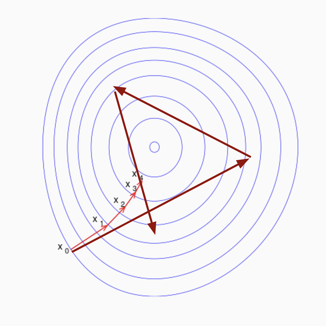
When we calculate the derivative for a given point in the loss landscape, we need to make sure we are not overly trusting of what that derivative tells us. Looking again at this diagram from earlier, we could take the inferred slope of the loss from the computed gradient at our location, and attempt to jump straight to the location that that would set the loss to zero along that plane. However, as seen in the example to the right represented in the thicker red lines, that would overshoot our desired minimized loss value and bounce around more than is desired. If we were to continue that process, we may never reach the minimum point in the center where overall error is most greatly reduced, because with every step we are likely to overshoot it rather than converging.

In this diagram, the use of a learning rate is shown through the smaller iterations on the thinner light red lines, where we move by a few percentage points of the amount predicted by the gradient to get closer and closer to the minima iteratively.

With all these pieces in place, we are now ready to start testing our network!

Validating on Boolean test cases

To re-iterate from above, the basic set of test cases we are targeting are to see if our network can learn basic boolean logic. We have test cases representing three models we want to train:

Boolean MUST
Boolean AND
Boolean OR

Each set of labels will be used to train a different network, and the tests will be setup and executed in a repeated table-driven style with the following cases:

First we set up a basic network to test against with just an input layer and single output layer.

We iterate over the boolean test cases and assert that the network can learn the outputs in each case. The predictionTestBool function is a simple helper that asserts that the output of the network always matches the output of the labeled data for the corresponding boolean function.

A test case for the multi-layer network it set up the same way, just adding the hidden1 layer to the network within the definition for the Layers array within the MLP.

Below is the output of these tests (with the Introspect function omitted for brevity). We can observe how the predictions trend toward the correct labels. The assertions in the test verify this, using fuzzy rounding logic with cutoffs to classify the network output one way to the other, and assert that it matches our expectations.

$ go test -v ./neural -run TestMLPMultiLayerBool
=== RUN   TestMLPMultiLayerBool
=== RUN   TestMLPMultiLayerBool/must
    mlp_test.go:114: input: [0 0], prediction: [0.12680678], label: [0]
    mlp_test.go:114: input: [0 1], prediction: [0.10898689], label: [0]
    mlp_test.go:114: input: [1 0], prediction: [0.8846526], label: [1]
    mlp_test.go:114: input: [1 1], prediction: [0.8737482], label: [1]
=== RUN   TestMLPMultiLayerBool/and
    mlp_test.go:114: input: [0 0], prediction: [0.03306453], label: [0]
    mlp_test.go:114: input: [0 1], prediction: [0.09745012], label: [0]
    mlp_test.go:114: input: [1 0], prediction: [0.1063798], label: [0]
    mlp_test.go:114: input: [1 1], prediction: [0.8444925], label: [1]
=== RUN   TestMLPMultiLayerBool/or
    mlp_test.go:114: input: [0 0], prediction: [0.08692269], label: [0]
    mlp_test.go:114: input: [0 1], prediction: [0.95728356], label: [1]
    mlp_test.go:114: input: [1 0], prediction: [0.9525525], label: [1]
    mlp_test.go:114: input: [1 1], prediction: [0.97686994], label: [1]
=== RUN   TestMLPMultiLayerBool/xor
    mlp_test.go:114: input: [0 0], prediction: [0.028652104], label: [0]
    mlp_test.go:114: input: [0 1], prediction: [0.9467217], label: [1]
    mlp_test.go:114: input: [1 0], prediction: [0.04812079], label: [0]
    mlp_test.go:114: input: [1 1], prediction: [0.9651075], label: [1]
--- PASS: TestMLPMultiLayerBool (0.00s)
    --- PASS: TestMLPMultiLayerBool/must (0.00s)
    --- PASS: TestMLPMultiLayerBool/and (0.00s)
    --- PASS: TestMLPMultiLayerBool/or (0.00s)
    --- PASS: TestMLPMultiLayerBool/xor (0.00s)
PASS
ok  	github.com/kujenga/goml/neural	0.243s

Validating on MNIST

Now that we have established that our network can learn basic boolean functions, let’s crank things up a few notches and take on the MNIST digits dataset.

Parsing MNIST

Before we can start working with the MNIST dataset directly, we need to parse it into a usable form. As mentioned above, the format of the data is a set of images represented as 28x28 pixel 2-dimensional arrays, where each value is a uint8 between 0-255 representing the color of the pixel. It also contains the corresponding label definitions, represented as uint8 values 0-9. The dataset is also stored in a rather unique binary format, which we handle as two separate parsing steps.

First, we create a parser for the binary idx dataset format, which returns the following parsed data structure from the binary files read out from disk.

Second, we create an mnist package which builds on IDX parser to read in the specific MNIST dataset using the capabilities of the IDX reader, and returns the following data structure for use in tests.

This parsing code is based directly on the MNIST spec and is all specified in the files linked to from the snippets just above, with corresponding test cases in those packages as well. Feel free to click through these code snippets into GitHub and explore the source code there if you are curious.

One-hot encoding

While we now have the raw data from the MNIST dataset, we still need to do a bit of transformation and data prep to be ready to train.

Neural networks are generally weaker when trying to predict a set of discrete outputs from a single neuron, if those outputs are not meaningfully correlated with the inputs from a numerical perspective.

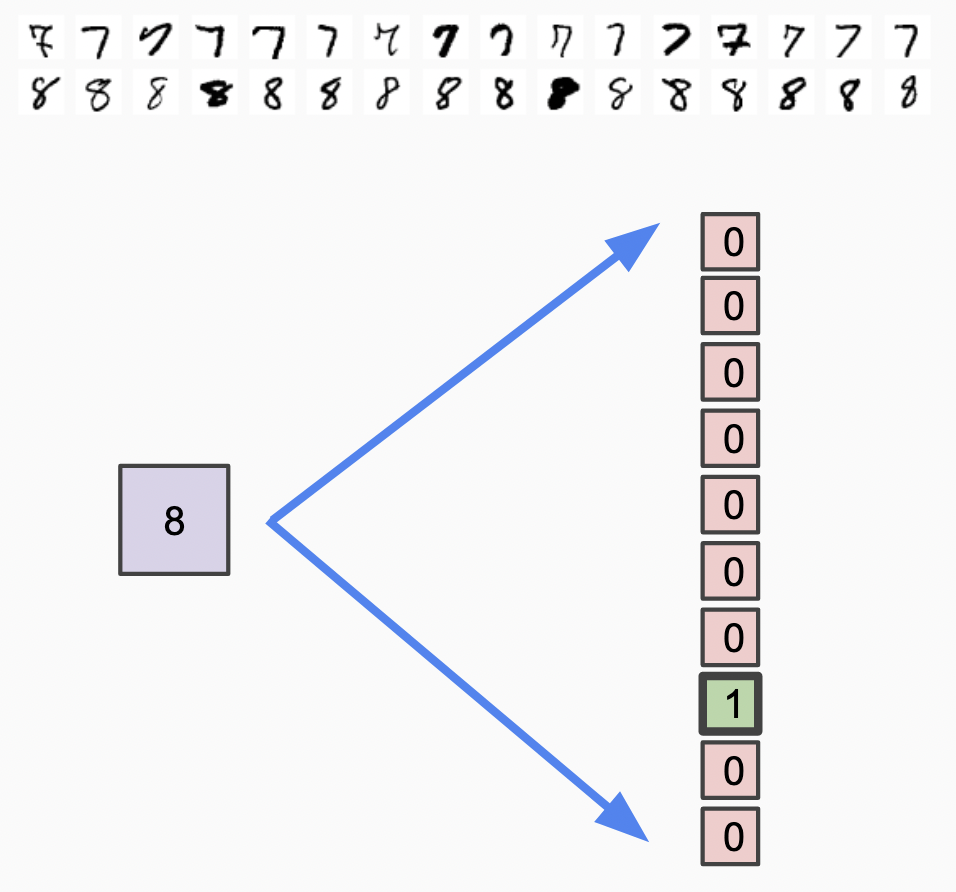
As an example of why this is the case, let’s look at the numbers 7 and 8. Numerically, they are right next to each other, meaning that the network outputs would need to be mathematically very close, while network outputs for 8 and 0 would need to be mathematically very far away. In terms of the visual representations of these numbers however, there is nothing about them which makes them closer together than any other pair of numbers in the range 0-9. Because our network is a mathematical combination of predictions, it would be difficult to have a network that could output a single numeric value quantized 0-9 to represent these digits.

One-hot encoding solves this problem. It uses a vector of binary values to make all the possible categorical outcomes independent of each other, as shown in this diagram, where “8” is mapped to a single “1” value within a vector, and all other values are set to 0. One-hot encodings are very useful for categorical variables, and that is what we will use here for representing MNIST.

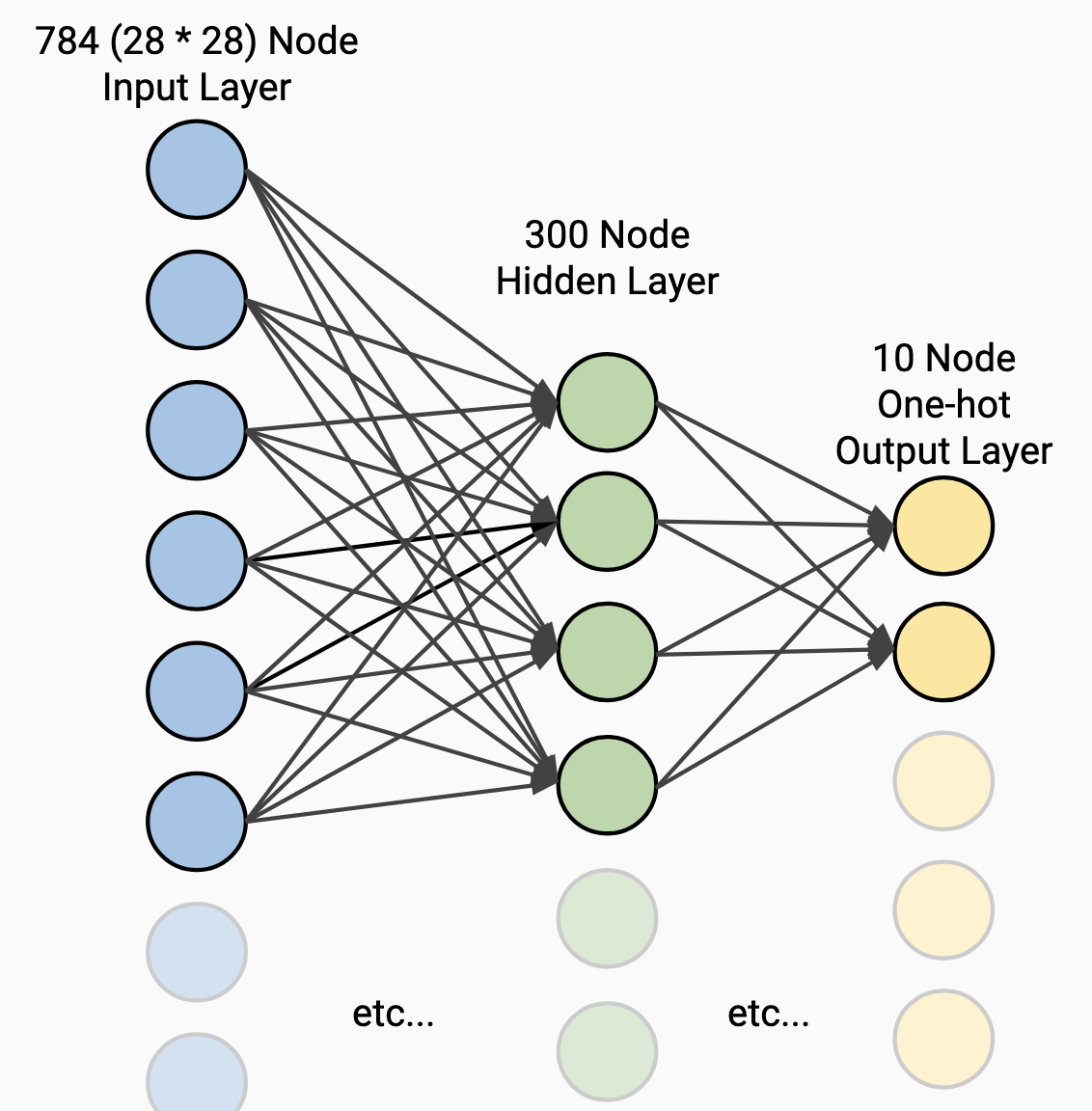
MNIST Network Architecture

Now that we have our dataset ready, we can start creating the architecture for our network. The following diagram depicts about what our network will look like conceptually, and is based on the network architectures documented on the MNIST page which compiles past results, maintained by Yann LeCun⁶.

One of these architectures is 2-layer NN, 300 hidden units, mean square error, which we will replicate here. It is worth noting though that modifications of this architecture with a different number of layers, layer sizes, etc. still can perform well!

MNIST Test cases

To implement our test cases for MNIST, in a similar manner to the boolean test cases above we lay out our network architecture for the MNIST network, execute the training process, and then validate our network performance. The input layer is the width of an array of all the pixels in a given 28x28 image from the dataset, and the output layer produces a vector with a one-hot encoding of the digit.

One key difference here is that we are training and validating on separate datasets, which are given to us separately by the MNIST dataset itself. This is a critical step forward towards tackling more realistic machine learning problems⁷.

For speed of execution in CI systems, the following test case limits the dataset size to 1/6 of what it normally would be, with 60k total examples. This is a trick that can be useful with very large datasets that can take a long time to train on. By using use a subset of your dataset that can be more quickly trained on you can iterate faster to get things functional, and then pull in the rest of the data later as you fine tune the architecture. Here our data isn’t really big enough to worry about that too much, but it is nice to have CI systems run a bit quicker when executing tests.

Validating our network performance is a bit more involved here than it was for the boolean test cases, as we need to compute an error rate for the network as a whole, rather than just asserting that it must be correct all the time as we did with the boolean test cases. Our test can then assert that the error rate is below a given threshold.

The predictionTestOneHot function does this for us. First we transform the one-hot output values into a digit representing the label from the dataset, and record whether or not it was a match. With those in hand, we can compute the ratio of correct results to incorrect results, giving us a score for how well the network did.

Running these tests locally, (with a slight modification to the source to remove the [:10000] slicing that just speeds up CI execution) we get the following output:

$ go test -v ./neural -run MNIST
=== RUN   TestMLPMultiLayerMNIST
    mlp_test.go:289: {Epoch:0 Loss:0.010991104}
    mlp_test.go:289: {Epoch:1 Loss:0.0065983073}
    mlp_test.go:289: {Epoch:2 Loss:0.0057215523}
    mlp_test.go:289: {Epoch:3 Loss:0.0051340326}
    mlp_test.go:289: {Epoch:4 Loss:0.004867792}
    mlp_test.go:145: one-hot predictions score: 0.9644
--- PASS: TestMLPMultiLayerMNIST (86.19s)
PASS
ok  	github.com/kujenga/goml/neural	86.409s

The score of 0.9644 we get here indicates we’re correct 96.44% of the time, equivalent to an error rate of 3.56%. This result is a bit better than the equivalent network architecture listed on the MNIST site! I would call that a definite success.

Conclusions and future exploration

At this point, we’ve walked through the creating a fully functioning neural network in Go from scratch, using just the tools given to us in the Go standard library.

Future blog posts may explore extensions of this network to provide additional functionality, such as batch and mini-batch approaches to the gradient descent phase.

We could also look at building on top of this network to target better MNIST performance through architectures like a Convolutional Neural Network which is particularly well suited for image-related tasks, and try to apply this network to additional image recognition datasets. Another avenue to explore is extending and refactoring this network to support Recurrent Neural Networks, which can be used on streams of data like text.

Another avenue to explore would be comparing the straightforward implementation we have here with approaches taken by other libraries, including Go-oriented libraries like [golearn][golearn], or some of the flagship libraries like tensorflow and pytorch which utilize a unique model to have the same code be runnable by a variety of execution backends like GPUs.

These may be topics for future posts! If you’ve made it this far, thanks for following along! I hope you found this helpful in gaining a deeper understanding of the basics of neural networks.

If you have any questions, comments, or other feedback, I would love to hear it in the comments below!

Resources

Source code for this project can be found here: https://github.com/kujenga/goml and the corresponding documentation is available here: https://pkg.go.dev/github.com/kujenga/goml

This post is based on a talk given for Boston Golang in Sept. 2021, the slides for which can be found here: Building a Neural Network in Go

This is a list of references I found useful in exploring the topics covered in this post, which can be delved into for further learning:

The Backpropagation explained YouTube series by Deeplizard is a great reference to go into even more detail on the concept and math behind the derivation process for backpropagation.
Make Your Own Neural Network is a fantastic book/e-book by Tariq Rashid that goes into more detail and background on this topic, and creates a functional network written in Python, exploring additional applications of linear algebra as well.
Build an Artificial Neural Network From Scratch: Part 1 is a helpful blog post from KDNuggets for walking through a simplified example of single layer networks.
Creating a Neural Network from Scratch in Python is a simpler walk through of a single-layer network in Python.
The MNIST dataset documentation, originally from Yann Lecun, and also mirrored at: https://deepai.org/dataset/mnist

https://towardsdatascience.com/why-do-neural-networks-need-an-activation-function-3a5f6a5f00a provides a great explanation of why activation functions are critical to making a multi-layered network. ↩︎
https://developer.nvidia.com/blog/mixed-precision-training-deep-neural-networks/ ↩︎
https://go.dev/blog/generics-proposal ↩︎
This article walks through examples of different loss functions: https://www.theaidream.com/post/loss-functions-in-neural-networks ↩︎
https://www.analyticsvidhya.com/blog/2021/03/variants-of-gradient-descent-algorithm/ ↩︎
https://web.archive.org/web/20211125025603/http://yann.lecun.com/exdb/mnist/ (I am providing a link to the archive page here as the original website is observed to sometimes ask for credentials) ↩︎
For more complex problems, or any sort of model that is expected to be deployed in production systems, just having separate train and test sets is usually not enough. Keeping separate “holdout” sets that you do not look at at all, as well as approaches like cross-validation are common to avoid common pitfalls with over-fitting to training data. You can read more about cross-validation here: https://towardsdatascience.com/what-is-cross-validation-60c01f9d9e75 ↩︎